Hellinger Mean

The Hellinger Mean compares how far the avatars' distributions are from a held-out half of the original dataset with how far the two halves of the original dataset are from each other. For interpretability, it uses the natural variability of the data as a reference.

For both comparisons, it computes the Hellinger distance variable by variable, where Hellinger distance measures the divergence between two probability distributions (0 = identical, 1 = completely different).

This metric applies to both categorical and continuous variables. For continuous variables, the Hellinger distance is estimated using histogram binning, while for categorical variables, it is directly computed from observed frequencies.

Working half (WO), holdout half (HO), working avatars (WA)

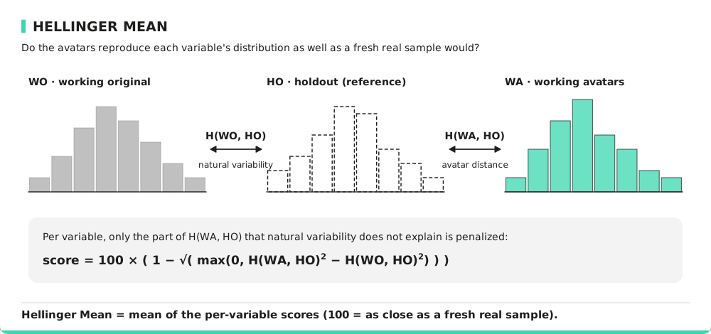
This is a reference-based metric: it compares the anonymization (WO vs its avatars WA) against the natural variability of the real data (WO vs a held-out reference HO).

• WO — working half original: the part of the original data that is anonymized.
• WA — working avatars: the avatars generated from WO.
• HO — holdout half original: a second, untouched sample of real records, used only as a reference.

On datasets large enough (by default ≥ 500 rows) a real holdout is set aside before anonymization; on smaller ones an approximate holdout is drawn by randomly splitting the data when the metrics are computed. See the "Evaluation with a holdout reference" section in the Technical Assessment report.

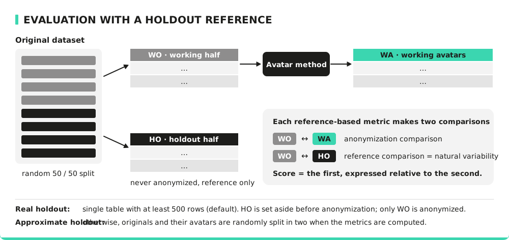
Comparison Strategy (Holdout)

To compute the final score returned to the user, we perform the following steps:

1. Obtain the working half WO and a disjoint holdout half HO from the real data (a real or approximate holdout — see the note above).
2. Take the working avatars WA, generated from WO.
3. For each variable, compute the Hellinger distance between WO and HO (reference distance: the natural variability).
4. For each variable, compute the Hellinger distance between WA and HO (avatar distance). Both distances are measured against HO, because the avatars are generated from WO and inherit its sampling error.
5. Score each variable as 100 × (1 − √max(0, avatar_distance² − reference_distance²)), then average the scores over the variables (see the formula below).

Interpreting the Hellinger Mean

• The closer to 100, the more avatars preserve the natural variability of the dataset.
• Values close to 100 indicate that avatars differ from original data as much as original data differ from each other — good signal retention.
• Values below 100 indicate that avatar distributions diverge more from original distributions than the natural variability would suggest — signal degradation.

Example

Consider a variable where the reference distance (between the two halves of the original data) is 0.05, and the avatar distance is 0.10. The part not explained by natural variability is √(0.10² − 0.05²) ≈ 0.087, so the variable scores 100 × (1 − 0.087) ≈ 91. An avatar distance equal to the reference distance would score 100.

Metric Specificity

Advantages:

• Captures the overall shape of distributions for both continuous and categorical variables.
• Uses the dataset's own natural variability as a reference, making the result more interpretable than a raw distance.
• Provides a bounded score between 0 and 100.

Limitations:

• Sensitive to the choice of binning when estimating distributions for continuous variables.
• May not fully capture local distribution differences.
• Can be impacted by sample size variations between datasets.

Formula

For one variable with probability mass functions $p$ and $q$ over the same bins $b$:

$$H(p, q) = \frac{1}{\sqrt{2}} \sqrt{\sum_b \left(\sqrt{p_b} - \sqrt{q_b}\right)^2}$$

For each variable $v$, the avatar distance is measured against the holdout, and only the part that the natural variability does not explain is penalized:

$$\text{score}_v = 100 \times \left(1 - \sqrt{\max\!\left(0,\; H(WA, HO)^2 - H(WO, HO)^2\right)}\right)$$ $$\text{Hellinger Mean} = \frac{1}{V} \sum_{v=1}^{V} \text{score}_v$$

Numeric variables are binned on a common grid of $\min\big(200, \max(20, \operatorname{round}(\tfrac{3}{4}(\max - \min)))\big)$ bins: equal-width bins, or equal-count bins when the values are significantly skewed. Categorical variables use their observed frequencies.

How to Improve This Metric?

To improve the Hellinger Mean score, you can adjust parameter k to help align distributions more accurately. You can also apply weighted projections by assigning higher importance to critical variables during data generation. Finally, you can use targeted data processing by applying transformations based on variable characteristics.