Kolmogorov-Smirnov

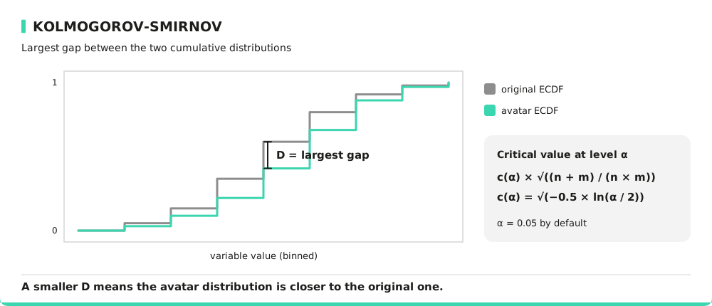
The Kolmogorov-Smirnov (KS) test is a non-parametric statistical test that compares two empirical cumulative distribution functions (ECDFs) to determine whether they originate from the same distribution. It calculates the maximum absolute difference between the ECDFs of the original and synthetic datasets.

The KS test is particularly useful for datasets with small sample sizes. In the implementation, the cumulative distributions are computed on the same bins as the other univariate metrics (see the formula below).

Interpreting Kolmogorov-Smirnov

The KS test provides a p-value that indicates whether the null hypothesis (the distributions are identical) can be rejected:

• p > 0.05: No significant difference between distributions.
• p < 0.05: Suggests the synthetic data differs from the original distribution.

Note: The alpha risk in a statistical test is the probability of incorrectly rejecting the null hypothesis when it is actually true. In simple terms, it means detecting an effect or a difference that does not actually exist. For example, in a medical trial, an alpha risk of 5% means there is a 5% chance of concluding that a treatment works when it actually has no real effect. Lowering alpha reduces this risk but increases the chance of missing a real effect.

A smaller KS statistic implies better similarity.

Example

Consider a dataset with a customer transaction amount variable. The KS test helps determine if the synthetic data maintains the same cumulative distribution. If the synthetic dataset underestimates high-value transactions, the KS statistic will be larger, indicating a divergence from the original data.

Metric Specificity

Advantages:

• Comes with a statistical decision threshold, making it useful for small datasets.
• Can detect subtle differences in cumulative distributions.

Limitations:

• More sensitive to small sample variations.
• Less intuitive than bounded metrics like Hellinger distance.

Formula

With $p$ and $q$ the binned distributions of the variable in the original ($n$ values) and avatar ($m$ values) data, and $F$, $G$ their cumulative sums:

$$D = \max_b \left| F_b - G_b \right| \qquad D_{\alpha} = c(\alpha) \sqrt{\frac{n + m}{n \, m}}, \quad c(\alpha) = \sqrt{-\tfrac{1}{2} \ln\!\left(\tfrac{\alpha}{2}\right)}$$

The distributions are considered different at level $\alpha$ (0.05 by default) when $D > D_{\alpha}$. Numeric variables are binned on a common grid of $\min\big(200, \max(20, \operatorname{round}(\tfrac{3}{4}(\max - \min)))\big)$ bins: equal-width bins, or equal-count bins when the values are significantly skewed. Categorical variables use their observed frequencies.

How to Improve This Metric?

To reduce the KS statistics of Kolmogorov-Smirnov test and enhance similarity, you can adjust parameter k to help align distributions more accurately. You can also apply weighted projections by assigning higher importance to critical variables during data generation. Finally, you can use targeted data processing by apply transformations based on variable characteristics.