Mutual Information

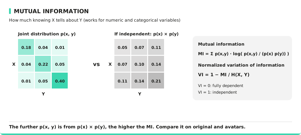
Mutual Information (MI) measures the dependency between two variables by quantifying the amount of information gained about one variable by knowing the other. Unlike Pearson correlation, MI works with both numerical and categorical variables. It is based on probability distributions rather than direct correlations allowing to capture non-linear dependencies.

Mathematically, MI is defined as:

$MI(X, Y) = \sum_{x \in X} \sum_{y \in Y} p(x, y) \log \left( \frac{p(x, y)}{p(x) p(y)} \right)$

where:

• $p(x, y)$ is the joint probability mass function (PMF) of $X$ and $Y$.
• $p(x)$ and $p(y)$ are the marginal PMFs of $X$ and $Y$.

Variation Information (VI) is a derived measure from MI, which normalizes dependency values between 0 (full dependency) and 1 (complete independence). Mathematically, VI is defined as:

$$VI(X, Y) = 1 - \frac{MI(X, Y)}{H(X, Y)}$$

where $H(X, Y)$ is the joint Shannon entropy of $X$ and $Y$:

$$H(X, Y) = - \sum_{x \in X} \sum_{y \in Y} p(x, y) \log p(x, y)$$

Interpreting Mutual and Variation Information

• High MI: Strong dependency between variables.
• Low MI: Weak dependency.
• VI = 0: One variable fully explains the other.
• VI = 1: The variables are completely independent.

Example

Consider a dataset with two variables:

• "Hours Studied" (X)
• "Exam Score" (Y)

In the original dataset, suppose Mutual Information between these variables is 0.85, indicating a strong relationship.

However, after transformation, if MI drops to 0.40, it suggests that a significant amount of information is lost, making the transformed dataset less reliable for predicting exam scores.

For Variation Information:

• If $VI_{\text{original}} = 0.2$ and $VI_{\text{transformed}} = 0.6$, it means that the transformed dataset has weakened the dependency between hours studied and exam scores.

Metric Specificity

Advantages:

• Unlike Pearson correlation, works for categorical and numerical data.
• Detects non-linear relationships.
• Not affected by outliers.

Limitations:

• Computationally more intensive.
• Harder to interpret than correlation coefficients (non linear scale).

Formula

With $p(x, y)$ the joint probability mass function of two variables (a 20 × 20 grid for two numeric variables; for a numeric and a categorical variable, a 20-bin histogram of the numeric variable within each category; observed frequencies for two categorical variables), and natural logarithms:

$$MI(X, Y) = \sum_{x}\sum_{y} p(x, y) \ln \frac{p(x, y)}{p(x)\,p(y)} \qquad H(X, Y) = -\sum_{x}\sum_{y} p(x, y) \ln p(x, y)$$ $$VI(X, Y) = 1 - \frac{MI(X, Y)}{H(X, Y)} \quad (VI = 0 \text{ if } H(X, Y) = 0)$$

To compare two datasets, the variation of information matrices are compared over the $p(p-1)/2$ pairs of variables:

$$\text{VI score} = \frac{2}{p(p-1)} \sum_{i > j} \left| VI^{\text{orig}}_{ij} - VI^{\text{avatar}}_{ij} \right|$$

How to Improve This Metric?

To enhance Mutual Information similarity, you can adjust parameter k to help align distributions more accurately. You can also apply weighted projections by assigning higher importance to critical variables during data generation. Finally, you can use targeted data processing by apply transformations based on variable characteristics. Please consider using alternative metrics (e.g., mutual information) if the data contains non-linear relationships or categorical variables.