Time Series Data

Time series data is a specific type of dataset where a variable is recorded multiple times over a given period. Examples include sensor readings, financial data, and medical signals such as electrocardiograms (ECGs).

Unlike traditional tabular data, time series data consists of multiple records (rows) per individual. Crucially, valuable insights often emerge from the evolution of values over time rather than from individual observations. For example, a sudden increase in blood pressure is only meaningful when analyzed in relation to previous readings.

A dataset typically contains multiple time series variables, each with distinct recording frequencies and durations. For instance, a vehicle may collect telemetry data from multiple sensors, each with different sampling rates.

If a time series variable contains only a few measurements per individual (e.g., fewer than five), it may be preferable to structure it as standard tabular data by assigning each measurement to a separate column or to use the multi table approach. The method described here applies to time series datasets with a larger number of time steps.

To be fully informative, time series data is often accompanied by static tabular data (e.g., patient age, gender, or device specifications). This complementary dataset is referred to as standard data and can be anonymized alongside the time series variables.

Avatars can accommodate multiple time series variables, even with differing lengths (time between first and last recordings) and frequencies (number of observations per second). However, when time series variables differ significantly in length and frequency, they should be stored in separate datasets.

Also note that the Time Series approach could be used embedded within a multi table anonymization (standard data being the parent patient data for instance and the time series itself being the child table.)

Scope of application

To ensure effective anonymization, time series data must meet the following conditions:

• Numeric Data Only: Time series variables must be numerical (categorical data is not supported).

• No Missing Values: Time series variables must not contain missing values, though missing values are allowed in the accompanying standard data.

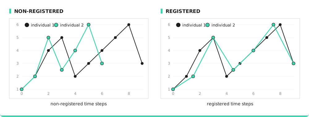
• Registered Time Series: Within a dataset, all time series must be registered, meaning:

  • Every variable has a value for each time step.
  • The time steps are the same across all variables.
  • Time series at a given time step must be comparable.

  We provide a tool to perform this registration prior to the anonymization.

  

• Regular Time Intervals: Time series data must be evenly spaced over time (i.e., fixed intervals between observations). We also provide a tool for this.

• Dataset Size Constraint: The number of individuals must be at least equal to the product of the number of time steps and the number of time series variables.

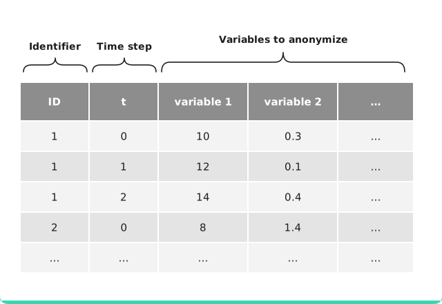
• Mandatory Identifier Variables: Time series data must contain:

  • An individual identifier that is the primary is caseof using time series approach with multi-table.
  • A time variable
  • The variables to be anonymized

  This flat data format follows a standard convention for time series representation.

Scalability:

This method can efficiently process datasets ranging from a few dozen to several thousands of time steps for multiple time series. Larger volumes of data are handled using a batch-parallelized approach, ensuring fast computation times.

Cyclic Data Specificities

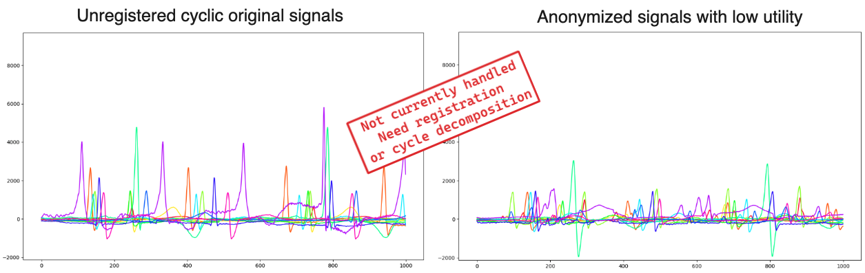
Cyclic data, where patterns repeat periodically (e.g., ECG signals), is not natively supported by this method. This is because cycles of different lengths across individuals lead to unregistered cycles, distorting the anonymized output.

To properly anonymize cyclic data, cycles should first be extracted and processed individually before reconstructing the full signal. If this preprocessing step is not feasible, anonymization at the cycle level is recommended.

Our scientific publication [^1] details an anonymization approach for ECG signals.

Output

Synthetic data return by this method have the following properties:

• Similar granularit:y Same number of time steps as after registration. Note that data could be unregistered afterwards using same given tools as the preprocess.
• Similar time patterns: Univariate information is preserved.
• Similar pattern clustering: Multivariate information is preserved.

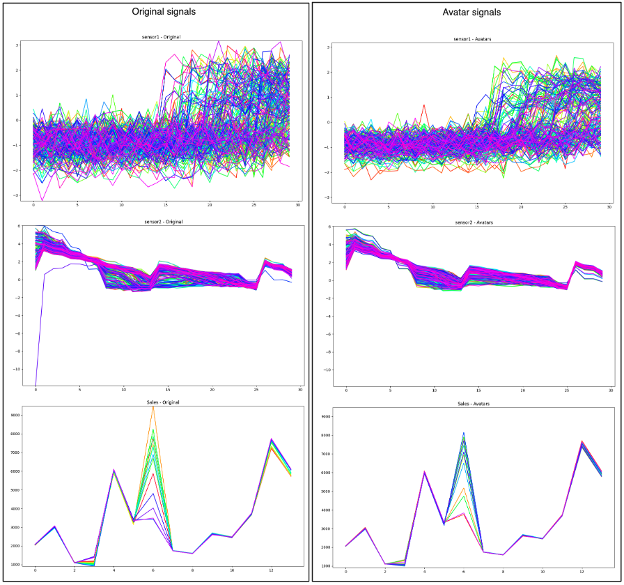Example of synthetic time-series output versus original data

Core Algorithm

To anonymize time series data, the overall process is similar to the one of standard tabular data described here, to the exception of the use of time series specific projection.

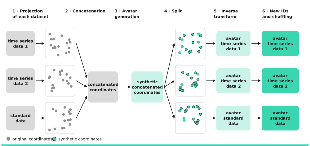
1. The first step is to project the data from each table in a multidimensional space where one row of data represents one individual. The standard data is projected like in the case of standard tabular data using a principal component method (Principal Component Analysis or Factor Analysis of Mixed Data). In order to preserve the relationships, trends and any other information that may exist between readings of a variable over time, specific projection methods (FFT, FPCA,...) are used for time series data. Currently, projection of such data is performed using Functional Principal Component Analysis (FPCA).

2. Once each dataset is projected into its own space, the projected data from the different datasets is concatenated in order to yield a single set of coordinates. Following concatenation, one row contains information coming from all datasets about a specific individual.

3. (Optional): In case of multiple time-series, if we are willing to keep multivariate information between time series we can either project all time series using Multivariate FPCA or by applying a PCA on concatenate coordinates.

4. After concatenation, synthetic coordinates are generated as explained here.

5. The synthetic coordinates are split so that projected variables are grouped according to the input datasets

6. The projection is reverse-transformed so that the synthetic data is expressed in its original form.

7. Finally, individual identifiers are re-generated and datasets shuffled

Example Usage

For a hands-on walkthrough of time series table anonymization, check out our Python notebook tutorial:

👉 Time Series Tutorial