Relational Database

Relational data refers to multiple tables with hierarchical relationships between them. This structure is referenced as Multi-table data.

A simple tabular anonymization approach applied independently to each table would be insufficient. Indeed, both privacy and utility depend not only on the individual tables but also on the relationships between them. For easy and effective handling of this data structure, we have developed a dedicated framework. This framework ensures the protection and preservation of inter-table relationships while maintaining data utility and privacy within each table.

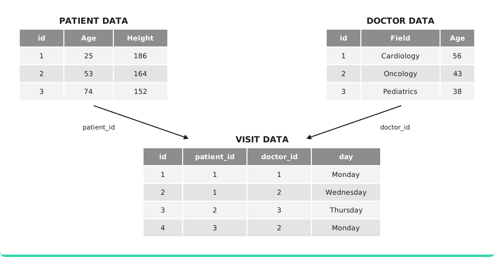
Example of structural database with 3 tables. Inter-table privacy risk is illustrated with patient 1 being the only one having 2 visits. Inter-table utility is illustrated with women having on average more visits than men.

Scope of application

The multi-table anonymization method shares the same scope as the single-table approach, meaning it supports the following data types:

Supported Data Types:

• Continuous variables (integer or float)
• Textual categorical variables (no matter the number of categories)
• Numeric categorical variables
• Boolean values
• Dates
• Missing data (the original distribution pattern of missing values will be preserved)

Specificity:

• all tables should contain one primary key
• all tables should be linked to another table using a primary key and a foreign key
• primary key should be one column and not a combination of multiple columns Scalability:
  This method can efficiently process datasets ranging from a few dozen to several billion records. Large volumes of data are handled using a batch-parallelized approach, ensuring fast computation times.

However, modeling the relationships between tables requires additional constraints to be met to ensure both privacy protection and structural consistency.

Each table must contain at least one identifier variable, known as a primary key, which holds a unique value for each row. Relationships between tables are established through foreign keys, which are identifier variables that reference the primary key of another table. Unlike primary keys, foreign keys do not need to be unique within their table, allowing multiple rows to link to the same referenced entity.

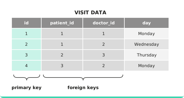
example of primary key and foreign key in a child table

Output

Such as Single Tabular anonymization, avatars from Multi-table anonymization have the following properties with regard to the original data:

• Same structure: Same number of variables with the same encoding and variable names.
• Same granularity: Same number of records (1-for-1 mapping).
• Similar aggregates: Expect similar averages, sums, medians, etc., across all variables.
• Similar links: Similar correlations between variables.
• Similar clustering properties: Multivariate information within the dataset is preserved.

But also:

• Similar inter-tables relationships: Multivariate information between tables is preserved.

Core algorithm

Definitions

We call parent table, the table having its primary key referred to in the other table. We call child table, the table having a foreign key referring to the other table. Finally, we call individual table a table where each row refers to a unique individual. In our example above, PATIENT_DATA and DOCTOR_DATA are individual tables. A link is defined between a parent table with a primary key and a child table with a foreign key referring to this primary key.

Algorithm

The anonymization of a multi table database is performed on each link between tables starting from top to bottom.

The top table is defined as the one with no parent table. For each link, the process is achieved in three main stages.

• Enrichment
• Avatarization
• Matching

For each link between tables (e.g. between PATIENT_DATA and VISIT_DATA):

1.Enrichment

Broadcast the information of the parent table in the child table. The join is based on parent table primary key and child table foreign key referring to the parent table.

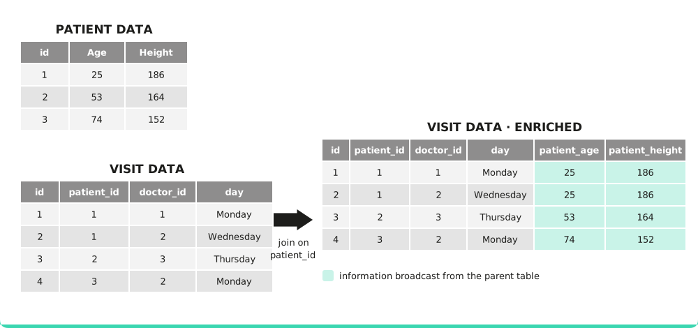
Illustration of enrichment step performing bottom information broadcast.

2.Avatarization

• Anonymize parent table using tabular anonymization described here.
• Anonymize enriched child table also using tabular anonymization.

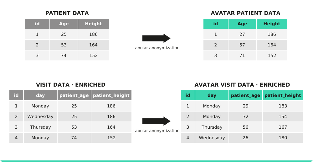
Illustration of tabular avatarization step for both parent and child enriched table.

3.Matching

Regarding the nature, the sensitivity and the volume of data we developed three methodology to perform a matching.

- minimum distance assignment

• Common information of avatar parent table and avatar child enriched table are transformed into coordinates using principal component method (Principal Component Analysis or Factor Analysis of Mixed Data)
• Distances are computed between coordinates from parent table and avatar child enriched table.
• Each record of the avatar child enriched table is associated with the closest record of the avatar parent table to recreate the parent foreign key in the avatar child enriched table.
• Columns broadcasted from parent table to child table are dropped to create the final avatar child table

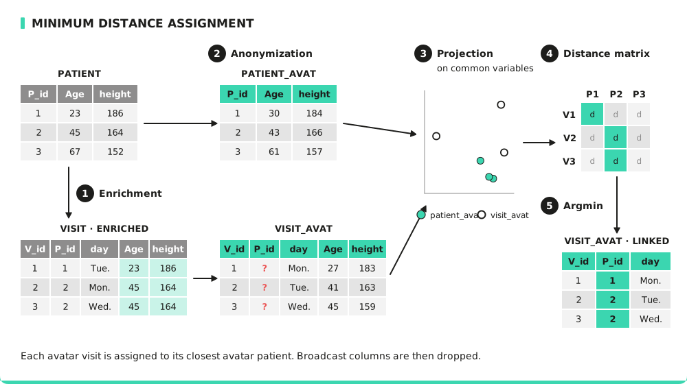
Illustration of minimum distance assignment methodology to recreate plausible match between parent and child table

- linear sum assignment

• Count of child events per parent id is avatarized in the parent table
• avatar rows of the parent table are duplicated according to avatarized count. This step is mandatory for the linear sum assignment algorithm as it applies to datasets of same shape.
• Common information of avatar parent duplicated table and avatar child enriched table are transformed into coordinates using principal component method (Principal Component Analysis or Factor Analysis of Mixed Data)
• Distances are computed between coordinates from parent table and avatar child enriched table.
• A linear sum assignment algorithm is applied to recreate the link between tables. each row from avatar parent duplicated table is associated with an avatarized visit following an optimization algorithm to minimize the total distance.
• Columns broadcasted from parent table to child table are dropped to create the final avatar child table

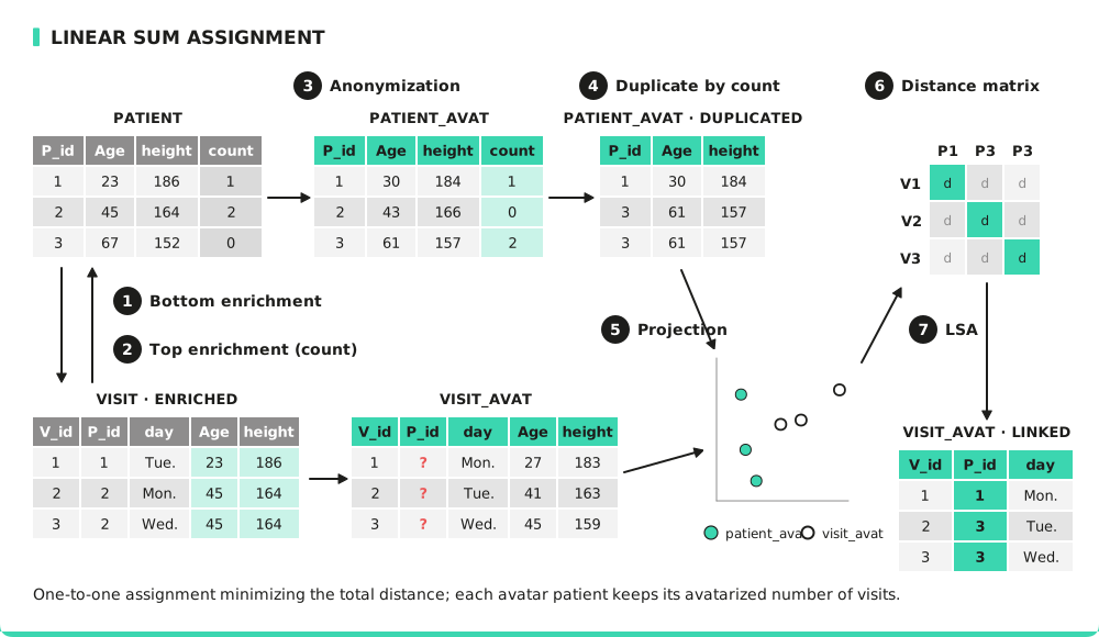
Illustration of linear sum assignment methodology to recreate plausible match between parent and child table

- original order assignment

• This methodology consists in keeping the exact same link as original thus avatarized visits of a specific individual will be reassigned to its avatar.

Use one of the three linking processes to generate plausible matches between parent table and child table information.

Advantages and drawbacks of different matching methods

Minimum distance assignment This is the methodology that ensures the highest level of privacy. It is faster than the LSA method, but has poorer preservation of aggregate distributions between tables, e.g. number of visits per patient.

Linear sum assignment This methodology shows the best balance between privacy and utility preservation. It preserves well aggregate distributions between tables while protecting rare events e.g. a patient having an abnormal number of visits. Because it is using an optimization algorithm, this methodology is also the slowest among the three.

Original order (sensitive) This methodology is fast and ensures a perfect preservation of aggregate distributions between tables. However, it is also the methodology that provides the least privacy guarantees.

Metrics computation

Since both privacy and utility are influenced not only by tables but also by the relationships between them, we calculate various approaches to assess risk at both the table level and their connections.

Privacy metrics

To evaluate privacy, we use the metrics defined here. Given the characteristics of the multi-table context, we have identified three distinct evaluation scenarios :

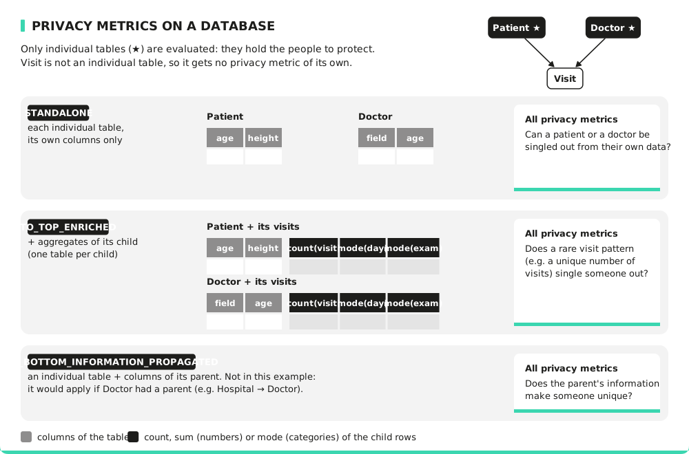
Individual-Level Table

For each individual level table (patient and doctor in our example) we assess privacy through different scenarios :

STANDALONE

This scenario assesses the privacy of a table by computing privacy metrics directly on the table.

TO TOP ENRICHED

This scenario evaluates the protection of individuals in a table considering the information from its child table. The individual-level table is enriched with aggregated information from its child table, and privacy metrics are computed on this enriched table.

Example

The patient table may show a low re-identification risk. However, if the linked visit table reveals that a specific patient has a unique number of visits, that count can put the patient at risk. By aggregating these visits information in the patient table, we can assess whether this additional information compromises patient privacy.

TO BOTTOM INFORMATION PROPAGATED

This scenario evaluates the protection of individuals in a table considering the information from its parent table. The individual-level table is enriched with information from its parent table, and privacy metrics are computed on this enriched table.

Example

Consider an hospital table linked to the doctor table. If a specific hospital has only one doctor specialized in a rare field, the specialty information propagated from the hospital table to the doctor table could make that doctor unique. By propagating this information, we can assess whether the relationship compromises the doctor's privacy.

As a table can have parents and children, multiple scenarios are considered.

Example

Below is a representation of the tables for which privacy metrics are computed following the different scenarios:

Signal metrics

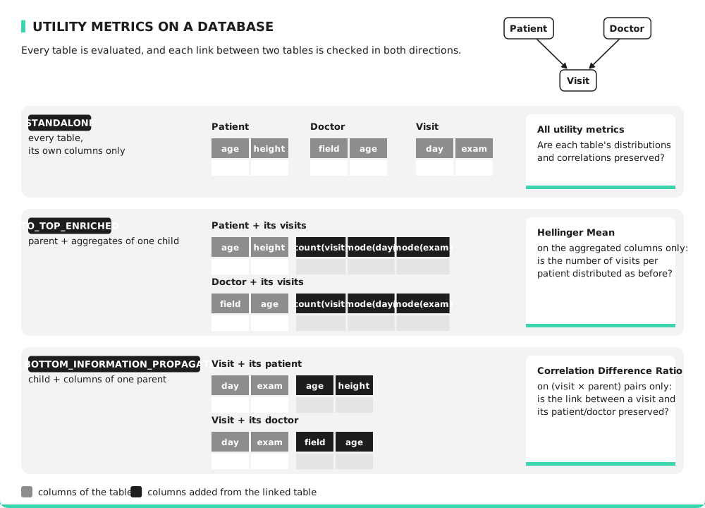
To evaluate signal, we use the metrics defined here. To evaluate the utility level of avatarization on the tables and relationships between table we defined 3 types of scenario :

Every table

STANDALONE : Signal metrics are computed for each table individually, without considering relationships with other tables.

Parent table

TO_TOP_ENRICHED : This scenario assesses the strength of the relationship between a parent table and its child table. The parent table is enriched with aggregated information from its child table, and we compute the hellinger distance. This process is repeated for each child of the parent table.

Child table

TO_BOTTOM_INFORMATION_PROPAGATED : This scenario evaluates the link between a child table and its parent table. The child table is enriched with broadcasted information from its parent table, and we compute the correlation difference ratio to assess the utility of the link.

As a table can have parents and children, multiple scenarios are considered.

Example

In our study case, here are the tables for which signal metrics are computed following the different scenarios :

Interpreting metrics

When evaluating privacy and signal metrics in a multi-table context, you must look beyond tables and consider the relationships between them. We provide a set of metrics to ensure you have the full context needed to judge anonymization quality.

While multi-table analysis can be complex, the following guidelines and summary table example will help you interpret your results and refine your avatarization parameters to balance privacy and utility.

The summary table highlights meta-metrics for a quick health check of your dataset. For a deeper dive into specific indicators, you can refer to detailed metrics results. This allows you to identify potential risks at a glance.

The rows represent the individual level table (the individuals you are protecting), while the columns represent all tables that could potentially leak information about those individuals.

Example

Table Name	Patient	Doctor	Visit
Patient	STANDALONE(Patient)		TO_TOP_ENRICHED(Patient, Visit)
Doctor		STANDALONE(Doctor)	TO_TOP_ENRICHED(Doctor, Visit)

Table Name	Patient	Doctor	Visit
Patient	90%		60%
Doctor		85%	90%

In the table above, the patient table has a high standalone privacy score of 90%. However, when analyzed with the visit table, the score drops to 60%.

tip

Improve Your Results

If you notice a significant drop in privacy due to relationships between tables, consider the following adjustments:

• Change the Matching Method: Try using a different assignment method, such as linear sum assignment or minimum distance assignment, to see if it better balances privacy and utility.

• Increase K: Increase the k parameter in the source of the risk (in this case, the visit table).

Example Usage

For a hands-on walkthrough of multi-table anonymization, check out our Python notebook tutorial:

👉 Multi-table Tutorial